D2L Chapter 4 Note

MLP

Why introduce nonlinearty:

Suppose

$\begin{aligned} \mathbf{H} & = \mathbf{X} \mathbf{W}^{(1)} + \mathbf{b}^{(1)}, \mathbf{O} & = \mathbf{H}\mathbf{W}^{(2)} + \mathbf{b}^{(2)}. \end{aligned}$

There is absolutely no fucking point of using H because it’s still a $\mathbf{X} \mathbf{W} + \mathbf{b}$ all along, and it’s equivalent to only one layer

So a nonlinearty thing is introduced by applying a nonlinear function to H:

$\mathbf{H} = \sigma(\mathbf{X}\mathbf{W}^{(1)}+\mathbf{b}^{(1)})$

Where $\sigma$ can be:

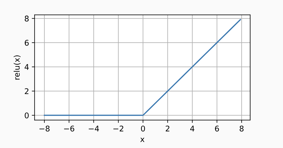
torch.relu(x)

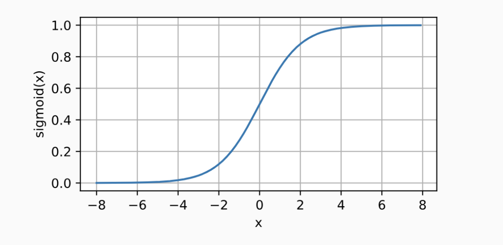
torch.sigmoid(x)

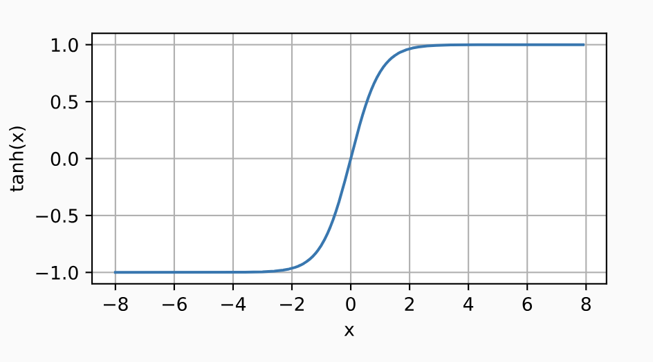
torch.tanh(x)

Implementation example:

OR:

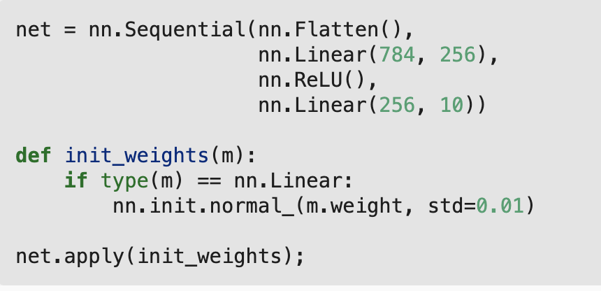
Other elements are exactly the same as softmax implemenation

Model selection

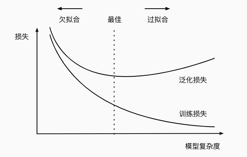
Fitting, Underfitting, Overfitting: Using way too much parameters and causing a model to become overfit to the training data is like using extra efforts to try to remember the whole textbook but fail to answer new questions in exam
Training vs Generalization
Training set + Validation set = Training process
Test set = Testing process

Weight decay

Literally R2 Regularization, after which:

$\mathbf L = L(\mathbf w,b)+\frac{\lambda}{2}||\mathbf w||^2$

and gradient is updated using

$\begin{aligned}\mathbf{w} & \leftarrow \left(1- \eta\lambda \right) \mathbf{w} - \frac{\eta}{|\mathcal{B}|} \sum_{i \in \mathcal{B}} \mathbf{x}^{(i)} \left(\mathbf{w}^\top \mathbf{x}^{(i)} + b - y^{(i)}\right).\end{aligned}$

Implemented as:

wd = lambda_to_be_used_that_specifies_penalty_level
trainer = torch.optim.SGD(
[{"params": net[0].weight, "weight_decay}: wd"}],
...
)
...
for i in range(epoch_num):
    for X, y in train_iter:
        trainer.zero_grad()
        l = loss(net(X), y)
        l.mean().backword()
        trainer.step()
        ...
    ...
...

Dropout

Forward & Backward propagation

Gradient vanishing & exploding

Gradient vanishing: in the chain, if only one chain’s gradient is zero or very small, the whole gradient chain will be very small because of it. Solution is to use ReLU

Gradient exploding: no convergence in optimizer

Initialization

Special initialization methods are used to solve the problem of symmetry, which means that if we initialize weights using the same value, model cannot distinguish different nodes, and the model cannot use its full computational power. Special methods include initializing weights using normal distriburion and Xavier initialization

Example: house price prediction

Data downloading & preprocessing: omitted

Define data input

all_features is the cleaned dataframe, n_train in the number of training rows to be used

().values enables the program to access the NumPy array

reshape(-1, 1): for the final reshaped train_labels, row is not specified (-1), col must be 1 (1).

train_features = torch.tensor(all_features[:n_train].values,dtype=torch.float32)
test_features = torch.tensor(all_features[n_train:].values,dtype=torch.float32)
train_labels = torch.tensor(
    train_data.SalePrice.values.reshape(-1, 1), dtype=torch.float32)

Definition of loss and net

what is the loss that MODEL USES is following standards.

What is the loss that WE USES is exactly calculated is defined by our own. Here we define loss as RMSE of logarithm value btwn actual and pred:

$\sqrt{\frac{1}{n}\sum_{i=1}^n\left(\log y_i -\log \hat{y}_i\right)^2}.$

clamp() is used to make everything in pred under 1 to be 1, for convenience of taking logarithm of it later

loss = nn.MSELoss()

def log_rmse(net, features, labels):
    clipped_preds = torch.clamp(net(features), 1, float('inf'))
    rmse_loss = torch.sqrt(loss(torch.log(clipped_preds), torch.log(labels)))
    return rmse.item()

in_features = train_features.shape[1]

def get_net():
  return nn.Sequential(nn.Linear(in_features,1))

Definition of train process

in each epoch, for each batch:

reset the gradient of trainer to be 0
feed X through net, calculate the training loss by using y
back propagate the loss
update the params

After each epoch, report the RMSE loss

Then begin next epoch by feeding each batch of training data again, repeat until an epoch number is reached

def train(net, train_features, train_labels, test_features, test_labels, num_epochs, learning_rate, weight_decay, batch_size):
    train_ls, test_ls = [], []
    train_iter = d2l.load_array((train_features, train_labels), batch_size)
    optimizer = torch.optim.Adam(net.parameters(),
                                 lr = learning_rate,
                                 weight_decay = weight_decay)
    for epoch in range(num_epochs):
        for X, y in train_iter:
            optimizer.zero_grad()
            l = loss(net(X), y)
            l.backward()
            optimizer.step()
        train_ls.append(log_rmse(net, train_features, train_labels))
        if test_labels is not None:
            test_ls.append(log_rmse(net, test_features, test_labels))
    return train_ls, test_ls

Use the model

Get the final training loss and get predictions on test data

net = get_net()

train_ls, _ = train(net, train_features, train_labels, None, None, num_epochs, lr, weight_decay, batch_size)
print(f'final log rmse：{float(train_ls[-1]):f}')

preds = net(test_features).detach().numpy()

Misc

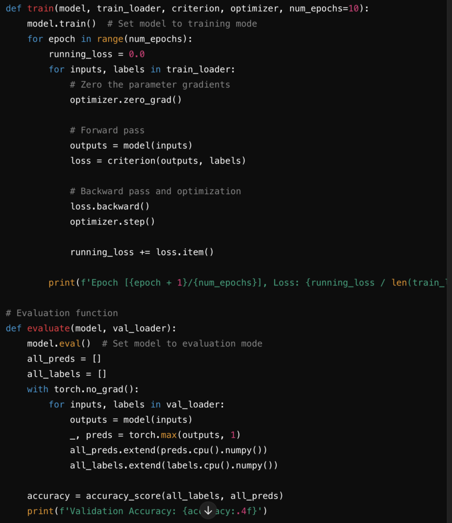
Setting the model to train / eval mode ensures the dropput and batchnorm layer function correctly, and other capability benefits. (Training mode will activate dropout, eval mode will disable dropout, things like this)

Each parameter’s gradients are calculated when updating the model from loss, calculated by partial derivative shits. The model prepares to calculate grad, unless no_grad is called, that’s why it is called in evaluation phase because in evaluation phase grads are not used

Parameters are updated using that gradient and learning rate when step() is called

After one batch of data completes its life cycle in the model, gradients need to be cleared to enable the model to learn from next batch, it is done using zero_grad

Post Views: 62

MLP